How We Calculate Win Probabilities

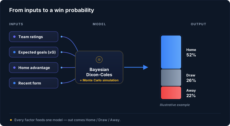
A walkthrough of the model pipeline that turns team ratings and form into home/draw/away probabilities.

A probability is not a prediction. When we say France has a 6% chance to win the 2026 World Cup, we are not saying France will win, and we are not saying they will lose. We are saying that when we simulate the tournament 50,000 times from the group stage forward, France lifts the trophy in roughly 3,000 of those runs. The other 47,000 belong to someone else. That distinction matters because every number on ParallaxEdge is a frequency over many possible futures, not a forecast of the one future that will actually happen.

The engine underneath is a Bayesian Dixon-Coles model. Each national team gets two parameters fit from historical match results: an attack rating that captures how many goals they tend to generate, and a defense rating that captures how many they tend to concede. The Bayesian part means we do not store a single number for each rating. We store a posterior distribution, a range of plausible values weighted by how consistent each one is with the data. Dixon-Coles is the Poisson-based scoreline framework from the 1997 paper of the same name, which we use because it handles low-scoring soccer results better than vanilla Poisson.

To turn ratings into a match forecast, we compute an expected goals value for each side. Home expected goals is a function of the home team's attack rating against the away team's defense rating, plus a home-advantage term. For neutral-venue World Cup fixtures that term is dialed down substantially, since neither side is truly at home. Away expected goals mirrors the calculation in reverse. Expected goals is the bridge between abstract team strength and a concrete probability. A matchup where one side projects to 2.1 xG and the other to 0.7 xG looks very different from a 1.4 versus 1.3 fixture, and the model needs to reflect that.

Those two expected goals values feed a bivariate Poisson distribution that produces a scoreline grid, a six-by-six matrix covering every result from 0-0 to 5-or-more versus 5-or-more. Each cell holds the probability of that exact scoreline. We then apply the Dixon-Coles correction to four cells in the low-scoring corner, 0-0, 1-0, 0-1, and 1-1, because raw Poisson systematically under-counts those results in real soccer data. To get the home-win probability we sum every cell where home goals exceed away goals. The diagonal gives us the draw probability. The cells below the diagonal give the away win.

A handful of teams in the 2026 field do not have enough historical match data to fit ratings directly. Cabo Verde, Curaçao, Haiti, Iraq and a few others fall into this category as first-time or rare World Cup participants. For those teams we use a prior derived from their current FIFA ranking, then calibrate that prior against the same statistical distribution the trained teams already occupy. The result is a rating with wider uncertainty bands than an established side, which is honest about what we know. The model does not pretend to have a confident read on a team it has barely seen.

After the scoreline grid is built, we run a marginal reconciliation step that rescales each outcome region so the published headline numbers stay internally consistent across the platform (this is internal to our own model — it has nothing to do with betting-market odds, which we never blend in). The home, draw, and away percentages you see on a match page are exactly the most-likely numbers from the underlying grid, and those same numbers feed the team strength scores and the tournament simulator. If you read Spain 49 percent against Saudi Arabia on the fixture page, you will see the same 49 percent reflected in every downstream view. There is no separate display layer quietly disagreeing with the math beneath it.

The point of all this machinery is calibration, not confidence. A model that says everything is 70 percent and then is right 70 percent of the time is more useful than a model that says everything is 95 percent and is right 60 percent of the time. We measure that calibration with the Brier score, covered in detail in the Understanding Brier Score lesson, which checks whether our stated probabilities match the long-run frequencies of what actually happens. The goal is straightforward: our 30 percent probabilities should hit roughly 30 percent of the time. That is the bar we hold ourselves to, and it is the bar we publish openly.